
Week 1: Can Linear Regression Predict Tomorrow’s Market?
Applying Machine Learning to Financial Data, Part 1 of 52

If you want to understand why this belong in my “Human in the Loop” series, skip to the end of the article.
This is the first of fifty-two weekly articles. Each one takes a single machine learning technique and turns it loose on financial data that anybody can obtain without paying for it. The series will climb, over the course of the year, from the plainest tool in the box to the architectures that sit behind the present excitement about artificial intelligence. We begin, deliberately, at the bottom of that climb, with ordinary linear regression, and we point it at the most unforgiving target there is: the daily return of the stock market.
The choice is not an accident. Before any of the clever methods arrive, it is worth establishing a discipline, because in this field the discipline matters a great deal more than the algorithm. A linear regression carried out with care will teach you more about financial machine learning than a transformer thrown together without it. So I want to start with a clear and slightly provocative question. Using nothing more than the recent history of returns and trading volume, can a simple linear model tell us whether the market will rise or fall tomorrow?
Saying the result out loud before we begin
It is only fair to state, before we touch the data, what we expect to find. Daily index returns behave very nearly like a random walk. Tomorrow’s move is governed for the most part by information that has not yet arrived, and the small remainder that might in principle be foreseeable is exactly the remainder that thousands of well-resourced participants are paid to compete away. If a model a hobbyist could build from a handful of past returns were able to call tomorrow’s direction reliably, that edge would have been bid out of existence long ago.
The honest expectation, then, is an out-of-sample fit hovering around zero, very possibly the wrong side of it, and a hit rate on direction that sits within a whisker of one half. I want to be plain that this is not the experiment failing. This is the experiment succeeding at telling us the truth. The whole value of the week lies in the method by which we reach that truth without deceiving ourselves, because it is the very same method that will keep us honest later, when the models are powerful enough to manufacture a thoroughly convincing illusion of skill.
The data
We use the daily closing price and trading volume of the S&P 500, retrieved through the yfinance library. It is free, it is everywhere, and it is entirely sufficient. The script caches what it downloads to a local file, so that the analysis can be reproduced even after the data provider has quietly changed something underneath it, which it will. It also records the exact span of dates it used, because a result you cannot date is a result you cannot trust.
One practical warning, which will return again and again across this series. The single most common way to produce a spectacular and entirely false result in financial machine learning is to allow information from the future to seep into the past. We will guard against it with something close to paranoia.
Building features without cheating
Every feature must be something we could genuinely have known at the moment we would have had to act on it. We are predicting the return from today’s close to tomorrow’s close, so every input has to be available by today’s close and not one second after it.
With that rule held firmly in mind, the features are modest and intuitive. We take the five most recent daily returns, the one that has just finished and the four before it. We add a five-day average of returns and two measures of recent volatility, over ten days and twenty-one, so the model can see both the recent drift and the recent turbulence. For volume we do not hand the model the raw figure, because volume creeps upward across the decades and a model given a steadily rising number will cheerfully mistake the mere passage of time for a signal. Instead we measure log volume against its own twenty-one-day average, which removes the trend and keeps the part that actually carries information, namely whether today was unusually busy.
The target is the next day’s return. In the code this is the return series shifted back by one position, so that the row labelled today carries tomorrow’s outcome. That single line is the precise spot at which most amateur backtests quietly cheat, and it earns both a comment in the source and a moment of your attention.
The rule that governs everything: respect time
Here is the point on which the entire series will insist, and it is worth stating without hedging. You must never shuffle financial data into a random training and testing split. The ordinary cross-validation that serves you so well on a collection of unrelated photographs is actively harmful here, because it trains on the future in order to predict the past and then reports back a fantasy.
So we split by time. The model learns on the earlier stretch of history and is judged on the most recent stretch, which it has never seen. For comparison and tuning we use walk-forward validation, expanding the training window forward through time, which is what scikit-learn’s TimeSeriesSplit provides. Any rescaling of the data is fitted on the training portion alone and then applied to the test portion, never the other way around, and we enforce this by binding the scaler and the regression together into a single pipeline, so that leakage becomes structurally impossible rather than merely something we tried to remember to avoid.
Baselines come before the model
A model is only ever as impressive as the dim-witted alternative it manages to beat. So before fitting anything, we write down three baselines. Predict zero every day. Predict the historical average return every day. Predict that tomorrow will simply repeat today. Each is trivial, and our regression must be measured against them rather than against some abstract notion of accuracy. A model that cannot beat “predict the average” has learned precisely nothing, and we want to discover that at once, rather than after we have talked ourselves into a comforting story.
What actually happened
With the apparatus in place, the results arrive quickly and without ceremony. The figures below come from a run over roughly five thousand trading days, with the final fifth held back for testing.
Begin with the baselines, because they frame everything that follows. Predicting the training mean every single day produced an out-of-sample fit of essentially zero, an R-squared of around -0.0002, which is what “no information, no error beyond the irreducible” looks like. More telling is the direction. Both the flat-zero and the flat-mean rules called the market correctly on 52.7 per cent of test days. They achieved this for the dullest of reasons: the market rose on more than half the days in the sample, so the rule “always guess up” is quietly rather good. Hold on to that number, 52.7 per cent, because it is the bar the model has to clear.
The model does not clear it. The linear regression returned an out-of-sample R-squared of -0.028. That minus sign is not a rounding artefact. It means the model performed worse than simply predicting the average, which is the signature of a model that has fitted noise: the relationships it learned on the training years did not survive into the test years, so applying them did active harm. Its directional accuracy was 50.7 per cent. The model, in other words, was beaten on direction by the most trivial rule available to us, the one that ignores the data entirely and always bets on a rise.
The walk-forward folds tell the same story, and they tell it in a more revealing way. They ran from -0.043 to -0.04 p, a mean a touch below zero and a spread more than twice the size of that mean. That instability is itself the finding. A genuine and durable signal would hold its sign from one window to the next. What we have instead is sampling noise wearing a different mask in each period.
The coefficients confirm it once more. After standardisation, every one of them sits at the third decimal place or smaller, with none standing out as carrying real weight. The largest, on yesterday’s return, is mildly negative, a faint scent of next-day mean reversion, far too weak to do anything with. The two volatility terms come out roughly equal and opposite, which is the classic appearance of two collinear features dividing a single weak effect between them rather than reporting two real ones.
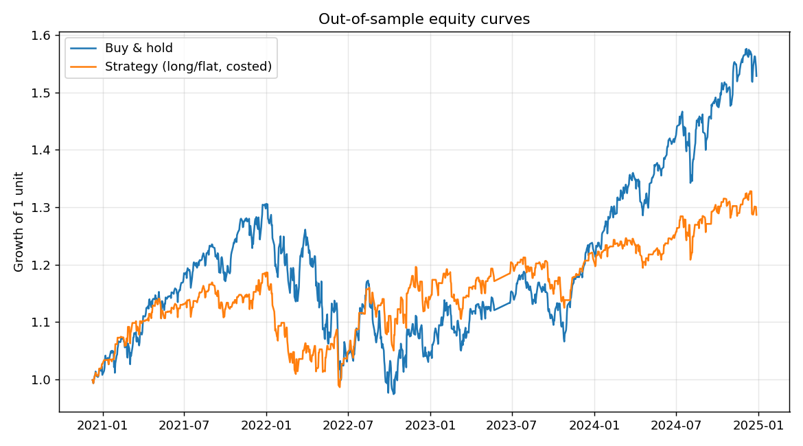
Then comes the test that actually settles the matter, the one with money in it. We let the model go long whenever it predicted a rise and sit in cash otherwise, and we charged a single basis point on every change of position. The strategy earned a Sharpe ratio of 0.49. Taken on its own that looks respectable, which is exactly the trap. Buying the index and holding it returned a Sharpe of 0.65 over the same window. The strategy underperformed doing nothing, and it did so after the gentlest possible allowance for costs. It spent stretches of time sitting in cash, missing the upward drift that is the market’s most dependable feature, and paid a toll for the privilege. The two equity curves below wander around one another for years before the trading rule quietly falls behind.
The one result that looks like good news, and why it is not
There is a loose thread to tie off, and it is the most instructive part of the whole exercise. When we fit the same model across the entire dataset and ask the formal statistical question, the regression comes back significant. The full-sample R-squared is 0.019 and the F-test returns a p-value of 0.009, comfortably past the one per cent threshold at which we conventionally declare an effect real.
A reader in a hurry would seize on this and announce that the model works after all. It does not, and reconciling the two findings is the lesson of the week.
The first point is the one we built the whole apparatus to respect. That significant R-squared was measured in-sample, on the same data the model was fitted to, including the very test period it then failed on. The minus zero point zero two eight was measured out-of-sample, on data the model had never met. A relationship can be statistically detectable in-sample and completely useless out-of-sample, and the gap between those two numbers is precisely the distance between a result and a delusion.
The second point is subtler and more important. Statistical significance and economic significance are not the same thing, and conflating them is one of the most expensive habits a person can carry into markets. With five thousand observations we have enough statistical power to detect an effect that accounts for under two per cent of the variation in daily returns. The p-value of 0.009 is reporting, quite truthfully, that a faint linear structure exists. The out-of-sample R-squared and the backtest are reporting, equally truthfully, that the structure is far too small to capture cleanly or to trade profitably once the world charges you to act on it. Both statements are correct at the same time. Markets are nearly efficient rather than perfectly so, and this is what “nearly” looks like when you write it down in numbers: real, detectable, and worthless.
There is also a small warning that the software will raise about the rank of the coefficient covariance. It is telling us that two of our features are very nearly the same thing, almost certainly the five-day mean of returns standing in for the lagged returns it is built from. It does not disturb the headline R-squared or the F-test, but it does mean the individual coefficient standard errors should not be read too closely. If clean per-coefficient inference were the goal, the redundant feature would come out. For our purpose, which is the overall verdict, the headline figures stand.
Why this is the right answer
It would have been the easiest thing in the world to present a tortured version of this analysis that produced a winner. Shuffle the data so the future leaks backward, scale before splitting rather than after, quietly try a few dozen combinations of features and report only the flattering one, leave out transaction costs altogether, and you can conjure a Sharpe ratio that would make a hedge fund blush. Every one of those moves is a real mistake that real people make with real money, and every one of them is a way of asking the data to lie to you. The discipline of this week exists to make each of them either impossible or visible.
The efficient-markets view predicts very nearly what we found. The readily foreseeable part of daily index returns, the part you could hope to catch with five lagged returns and a volume ratio, is close to nothing, because it is the cheapest edge imaginable and therefore the first to be competed away. The opportunities that do exist, to whatever extent they exist at all, live in richer data, in faster reactions, or in genuinely harder modelling, and we will meet a few of them as the year goes on.
What carries forward
The technique this week was disposable. The habits are permanent. A target built so the future cannot leak backward into it. Features that respect the moment of decision. Splitting by time, and validating by walking forward through it. Baselines written down before the model is fitted. An evaluation that ends with costs and a Sharpe ratio rather than beginning and ending with R-squared. Coefficients examined for stability across periods rather than admired in a single comfortable fit. And, underpinning all of it, a refusal to mistake a significant p-value for a useful one.
Carry these forward and the rest of the series rests on solid ground. Abandon them and no amount of architecture will rescue you, because a powerful model trained on a leaky setup does not fail loudly and helpfully. It succeeds, gloriously and falsely, which is by far the more dangerous outcome.
Next week we stay with regression but give it something with a fighting chance, explaining a single stock’s returns with the Fama and French factors. We shall see what changes when the right-hand side of the equation finally holds variables with a real economic claim on the left.
The complete, runnable script accompanies this article. It tries live data first, caches it locally, and falls back to a freely mirrored daily series, and then to a simulated one with realistic statistical properties, so that it runs anywhere. The figures quoted above come from a run over roughly five thousand trading days; run it on your own machine and the exact decimals will shift, but the shape of the result will not.
The full repository, including the mlfin core package, the test suite, and this article, lives at github.com/Oyetade/ml-finance-52. Clone it, run pip install -e ., and python run.py inside the Week 1 folder to reproduce every number above.
A note on how this was made, since this newsletter is partly about exactly that.
This project, and the code beneath it, came out of a working session with Claude, an AI assistant, and the collaboration is worth describing honestly because it was neither of the two caricatures people tend to reach for. It was not the AI handing me a finished codebase to ship under my name, and it was not me using the AI as a glorified autocomplete. It was something more like working with a capable, tireless engineering colleague who needed supervising.
The division of labour fell out naturally. The model was genuinely useful at the mechanical and the structural: scaffolding the repository, refactoring the shared logic into a clean installable package with its own tests, writing the leakage-proof split and the costed backtest once and properly so they could be reused across all fifty-two weeks, and catching that a careless GARCH parameterisation would make my synthetic fallback data explode before it ever reached a chart. It worked through the unglamorous discipline that good engineering actually consists of, the validation guards, the offline fallbacks, the reproducibility, without tiring of it, which is precisely the part a human is tempted to skimp on. But every judgement that mattered stayed with me. Which technique to apply, how to structure the series so it would still cohere at week fifty, whether a result was being framed honestly, and above all whether the thing was correct: those were mine, and the model was at its most useful when I treated its output as a draft to interrogate and test rather than an answer to accept.
The most instructive moments were the corrections in both directions. When the live data source was blocked, the AI quietly substituted a synthetic series and reported results from it, and it would have been easy to let those numbers stand; catching that, and insisting on real market data even when it was inconvenient to obtain, was the human keeping the work honest. Equally, the model pushed back usefully on my own loose thinking more than once, and querying its explanations line by line is how I made sure I understood the code I was about to put my name to rather than merely trusting it. The lesson I take from it, and the reason this newsletter exists, is that the value was not in the AI replacing the engineering but in compressing the distance between an idea and a working, tested implementation, on the firm condition that a human stayed in the loop to own the judgement and carry responsibility for what was shipped. The repository carries my name because the accountability is mine. The assistance simply let me do more of the work I actually wanted to do, and less of the work I didn’t.